Objectives:
Develop two simple image classification networks (1-bit and 32-bit) in Python.
Profile both networks and compare their results.
What you should know:
Welcome back! If you've been following along, this is the second part of our series dedicated to the practical implementation of Binary Neural Networks (BNNs). If you haven't had the chance yet, I highly recommend checking out the first part to grasp the foundational context before diving into the implementation phase.
Now, let's delve straight into the core of it!
Larq:
In order to implement a BNN, we can use a library called Larq that is based on Keras, which helps us implement a true binary network that actually operates on 1-bit rather 32-bit. Larq uses a highly optimized inference engine which utilizes various optimization techniques such as SIMD, multi-threaded parallelization and more. You can read more about their engine here.
Dataset and Pre-processing:
To keep things straightforward, we'll employ the MNIST dataset to train and assess both networks for an image-classification task.
In the code snippet provided below, we utilize the tf.keras.datasets.mnist.load_data() API to import the MNIST dataset. This API automatically loads the dataset, divides it into training and testing subsets, and distinguishes between the image features and their corresponding classification labels.
Following the dataset loading, the subsequent step involves reshaping the features. This is necessary to ensure that the networks can actually train on the data.
import tensorflow as tf
import larq as lq


# Data Pre-Processing
(train_images, train_labels), (test_images, test_labels) = tf.keras.datasets.mnist.load_data()

# Normalize pixel values to be between 0 and 1
train_images, test_images = train_images / 255.0, test_images / 255.0

# Reshape the images to the format (28, 28, 1) as the MNIST images are grayscale
train_images = train_images.reshape((60000, 28, 28, 1))
test_images = test_images.reshape((10000, 28, 28, 1))
Note: This step is the same for both networks as we will be using the same dataset for both networks.
Full-Precision:
The following code snippet showcases the layer depth configuration for the full-precision network. To ensure a fair comparison with the BNN, we maintain an identical depth for both networks. This approach aims to yield unbiased and directly comparable results between the models.
As we undertake a multi-class classification task using the MNIST dataset, the choice of activation functions in our neural network is crucial. Specifically, we employ the Softmax activation in the final output layer, which comprises 10 nodes, corresponding to the 10 distinct classes in the dataset. This setup directs the network to categorize each input into one of these ten classes.
Meanwhile, the Rectified Linear Unit (ReLU) activation function is utilized in the hidden layers. This choice optimizes the network's ability to learn complex patterns within the data, enhancing its performance in identifying and processing features for classification.
For the optimization technique driving the network's parameter updates during back-propagation, we implement the ADAM optimizer.
The network will run for 6 epochs with a batch size of 64.
# Defining the model structure
model = tf.keras.models.Sequential()

# The first convolutional layer with default TensorFlow layers
model.add(tf.keras.layers.Conv2D(32, (3, 3), activation='relu', input_shape=(28, 28, 1)))

model.add(tf.keras.layers.MaxPooling2D((2, 2)))
model.add(tf.keras.layers.BatchNormalization())

# The second convolutional layer
model.add(tf.keras.layers.Conv2D(64, (3, 3), activation='relu'))
model.add(tf.keras.layers.MaxPooling2D((2, 2)))
model.add(tf.keras.layers.BatchNormalization())

# The third convolutional layer
model.add(tf.keras.layers.Conv2D(64, (3, 3), activation='relu'))
model.add(tf.keras.layers.BatchNormalization())
model.add(tf.keras.layers.Flatten())

# Fully connected layers
model.add(tf.keras.layers.Dense(64, activation='relu'))
model.add(tf.keras.layers.BatchNormalization())

# Output layer, multi-class classification
model.add(tf.keras.layers.Dense(10, activation='softmax'))

# Compile and train the network
model.compile(optimizer='adam',
              loss='sparse_categorical_crossentropy',
              metrics=['accuracy'])

model.fit(train_images, train_labels, batch_size=64, epochs=6)
Binary Neural Network:
The code snipped below shows a very simple BNN, that is almost identical to the full-precision network mentioned above. This network will utilize Larq's API to define binary layers. The major differences between this network and the full-precision network mentioned above, is kernel_quantizer and input_quantizer arguments used in the layers.
These two arguments play a pivotal role, defining the methodology by which Larq will binarize the inputs from preceding layers and the weights of the kernel. Specifically, we opt for the Straight-Through Estimator (STE), as elaborated in part 1 of this series, to binarize these inputs and weights.
Moreover, the kernel_constraint argument assumes significance by constraining the kernel weights to binary values during parameter updates. This constraint is vital to ensure that the weights remain within the binary realm, aligning with the desired binary representation and preventing them from deviating beyond these binary values.
 Defning the model structure
# Following Larq's documentation model depth and parameters
model = tf.keras.models.Sequential()

# The first layer, only the weights are quantized while activations are left full-precision
model.add(lq.layers.QuantConv2D(32, (3, 3),
                                kernel_quantizer="ste_sign",
                                kernel_constraint="weight_clip",
                                use_bias=False,
                                input_shape=(28, 28, 1)))

model.add(tf.keras.layers.MaxPooling2D((2, 2)))
model.add(tf.keras.layers.BatchNormalization(scale=False))

# The second layer has both quantized weights and activations using the Straight-through-estimator sign activation technquie.
# Using straight-through-estimator to overcome undifferentiability issues
model.add(lq.layers.QuantConv2D(64, (3, 3), use_bias=False, input_quantizer="ste_sign",kernel_quantizer="ste_sign",kernel_constraint="weight_clip"))
model.add(tf.keras.layers.MaxPooling2D((2, 2)))
model.add(tf.keras.layers.BatchNormalization(scale=False))

# The third layer following the second layer
model.add(lq.layers.QuantConv2D(64, (3, 3), use_bias=False, input_quantizer="ste_sign",kernel_quantizer="ste_sign",kernel_constraint="weight_clip"))
model.add(tf.keras.layers.BatchNormalization(scale=False))
model.add(tf.keras.layers.Flatten())
# The fourth layer
model.add(lq.layers.QuantDense(64, use_bias=False, input_quantizer="ste_sign",kernel_quantizer="ste_sign",kernel_constraint="weight_clip"))
model.add(tf.keras.layers.BatchNormalization(scale=False))
# The fifth layer
model.add(lq.layers.QuantDense(10, use_bias=False, input_quantizer="ste_sign",kernel_quantizer="ste_sign",kernel_constraint="weight_clip"))
model.add(tf.keras.layers.BatchNormalization(scale=False))
#Output layer, multi class classification
model.add(tf.keras.layers.Activation("softmax"))


#Compile and train the network
model.compile(optimizer='adam',
              loss='sparse_categorical_crossentropy',
              metrics=['accuracy'])

model.fit(train_images, train_labels, batch_size=64, epochs=6)
Profiling:
To effectively profile both networks, we'll leverage Larq's built-in profiler, offering a convenient and efficient means of conducting neural network profiling. The following code snippet demonstrates the application of the profiler. An interesting feature is that the Larq profiler can be employed not only with binary networks but also with full-precision networks. Consequently, Larq needs to be imported even when working with a full-precision network, showcasing the versatility and utility of this profiler.
# Evaluate the network
lq.models.summary(model)
test_loss, test_acc = model.evaluate(test_images, test_labels)
Results and Analysis:
Full-precision:
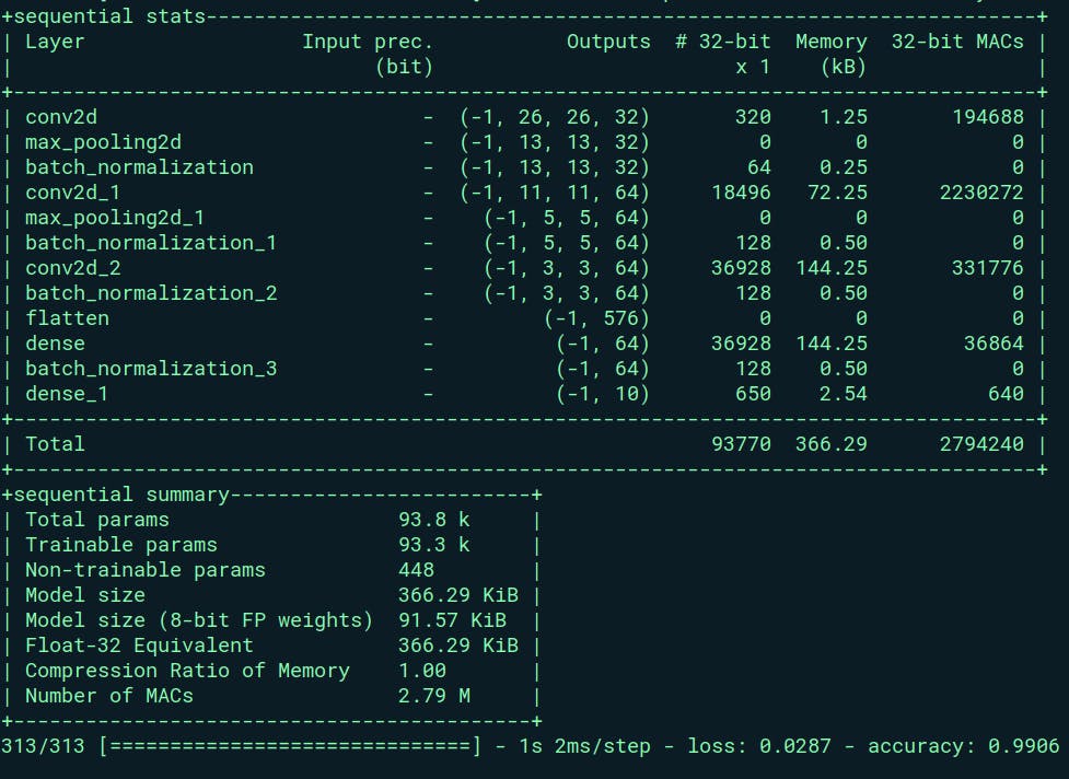
The captured information from Larq's profiler reveals essential details about the full-precision network. The network comprises a total of 93,770 parameters, encompassing weights, batch normalization, and other factors. Remarkably, the parameter size sums up to 366.29 KB, a relatively negligible size for contemporary computing systems.
During operations, the network performs 2,794,240 multiply-accumulate (MAC) operations, which involve dot operations and accumulation in an accumulator. The network exhibits outstanding performance, achieving a remarkable 99.06% accuracy on the dataset with a low loss of 0.0287. This high level of accuracy denotes commendable classification performance within the dataset.

Binary Neural Network:
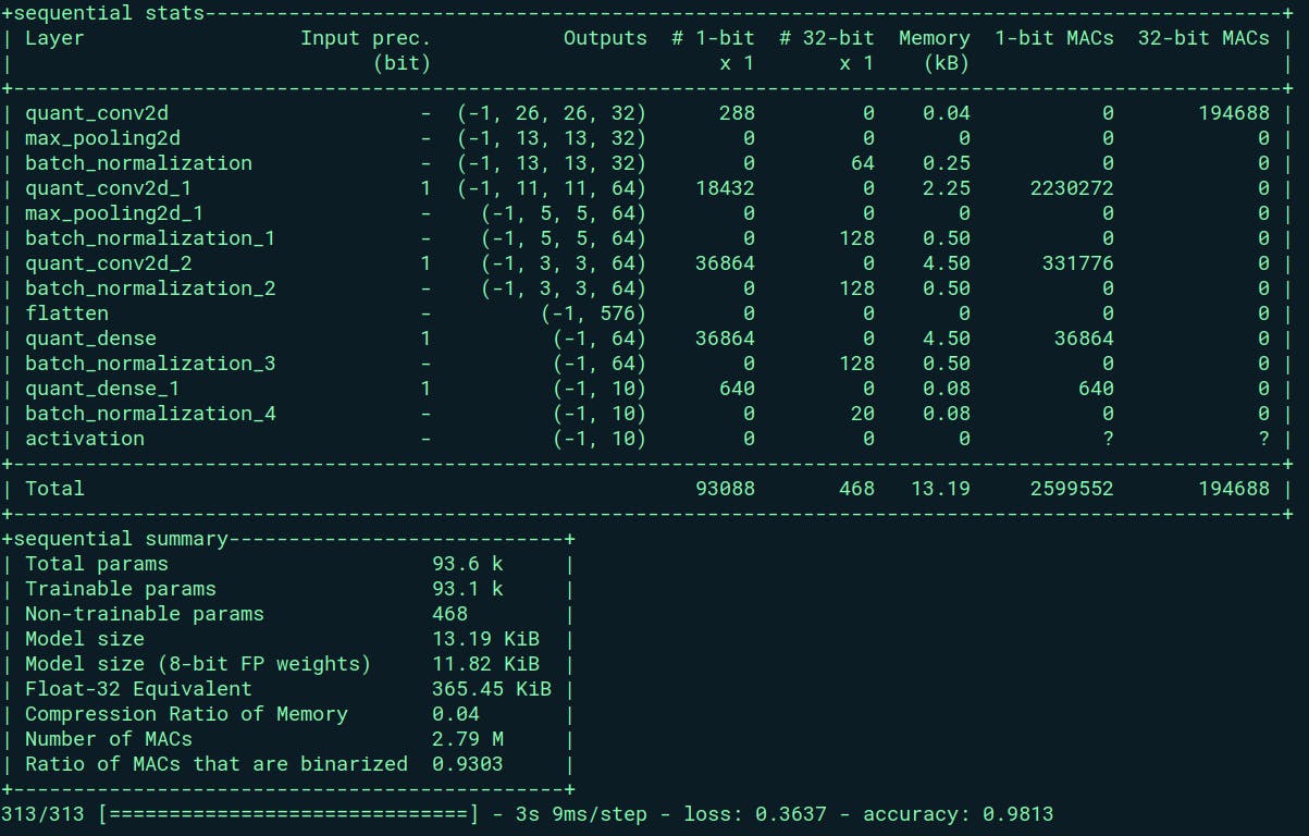
Transitioning to the binary neural network, we observe a remarkable reduction in resource utilization compared to its full-precision counterpart. This network comprises approximately 93,556 parameters, a figure comparable to the full-precision network.
Notably, a mere 468 parameters within this binary network remain in the 32-bit format, primarily stemming from batch_normalization parameters. However, the bulk of the parameters—comprising an impressive majority—are condensed to a 1-bit representation.
This reduction in parameter bit-width results in a striking decrease in network size. The total footprint of this binary network amounts to a mere 13.19 KB, signifying an exceptional reduction in resource consumption when compared to the full-precision network.
This is 96.45% reduction in memory size !!!!!!!!
An interesting observation is that approximately 93% of the Multiply-Accumulate (MAC) operations within the binary neural network are binarized. This holds substantial significance, particularly in hardware implementation. The transformation of heavy full-precision operations into basic XNOR operations within the binary network considerably accelerates computation. XNOR operations are notably faster and computationally less complex compared to their full-precision counterparts. This high percentage of binarized MAC operations underscores the efficiency gains achieved by employing a binary neural network, particularly in terms of hardware realization and computational efficiency.
However, it's essential to note a slight trade-off when adopting Binary Neural Networks (BNNs). Despite their resource efficiency and smaller footprint, BNNs often exhibit a marginal decrease in accuracy compared to their full-precision counterparts.
In this case, the accuracy achieved using the BNN on the same dataset registers at 98.13%, whereas the full-precision model achieved 99.06%. This translates to a 0.93% reduction in accuracy when transitioning from full-precision to one-bit representation.
This accuracy degradation stands as the primary drawback of BNNs. While they offer notable resource savings and computational efficiency, the shift from full-precision to one-bit representations tends to impact the network's overall accuracy.

Summary:
In this series exploring Binary Neural Networks (BNNs) compared to full-precision networks, we harnessed Larq, a Keras-based library, to develop and analyze two image-classification models using the MNIST dataset.
The full-precision network demonstrated exceptional accuracy, achieving 99.06% on the dataset with a relatively small parameter size of 366.29 KB. However, the binary neural network (BNN) showcased remarkable resource savings, condensing parameters to a mere 13.19 KB, marking a staggering 96.45% reduction in memory size. Additionally, 93% of Multiply-Accumulate (MAC) operations were binarized, elevating computational efficiency significantly.
Despite these efficiency gains, the BNN experienced a slight accuracy reduction of 0.93% compared to its full-precision counterpart. This accuracy trade-off remains a critical consideration when adopting BNNs, as the shift from full-precision to one-bit representation impacts overall accuracy.
Ultimately, while BNNs present an enticing prospect with their efficiency gains and smaller memory footprint, the trade-off in accuracy warrants careful consideration, particularly in scenarios where accuracy is paramount.
This exploration highlights the trade-offs between resource efficiency and accuracy, offering valuable insights into the practical implications of deploying binary neural networks in image-classification tasks.
In Part 3 of this series, we'll delve deeper into the application of binary neural networks (BNNs) by exploring their use in anomaly detection. Specifically, we'll train a binary neural network tailored for anomaly detection—an essential component in bolstering cyber-security measures, particularly in the realm of Intrusion Detection Systems (IDS).
